Quantum Protein Folding

A quantum computing approach to solving the protein folding problem using Qiskit. This project implements Variational Quantum Eigensolver (VQE) algorithm to predict the 3D structure of proteins based on their amino acid sequence.

Our implementation is inspired by and extends the methods described in
Protein Folding Problem: A Quantum Approach, and this repository: quantum-protein-folding-qiskit

• Overview
• Features
• Visualizations
• Requirements
• Installation
• Usage
• Documentation (Sphinx)
• Running Tests
• Adding Dependencies
• Project Structure
• How It Works
• Key Modules
• Contributing
• Authors
• License

🧬 Overview

Protein folding is one of the most challenging problems in computational biology. This project leverages quantum computing to explore protein conformations on a lattice model, using quantum optimization to find low-energy states that represent folded protein structures.

The implementation uses:

• Qiskit for quantum circuit construction and simulation
• VQE (Variational Quantum Eigensolver) for quantum optimization
• Hamiltonian formulation combining distance constraints, contact interactions, and backtracking penalties
• HP and MJ interaction models for residue-residue energies

✨ Features

• 🔬 Multiple interaction models: Hydrophobic-Polar (HP) and Miyazawa-Jernigan (MJ)
• ⚛️ Quantum backend support: IBM Quantum and local simulator
• 📊 Rich visualizations: 2D projections, interactive 3D plots, and animated rotations
• 📈 Result tracking: Detailed logging of VQE iterations, energies, and convergence

🎨 Visualizations

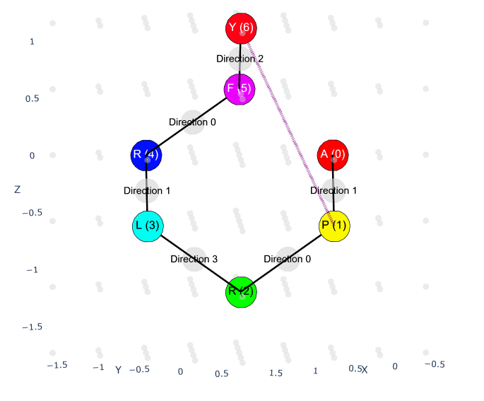
The quantum optimization produces protein conformations that can be visualized in multiple ways:

Interactive 3D Visualization

Click to view the interactive 3D visualization (HTML)

Rotating Animation

Animated 360° rotation of the folded protein structure

The visualizations show:

• Backbone chain (main chain beads) in one color
• Residue labels for each amino acid position
• 3D spatial arrangement on a discrete lattice
• Energy-minimized conformation from VQE optimization

📋 Requirements

• Python 3.12 or higher
• uv - Fast Python package and environment manager

🚀 Installation

1. Install uv

Choose one of the following methods:

Linux/macOS:

curl -LsSf https://astral.sh/uv/install.sh | sh

Windows (PowerShell):

powershell -ExecutionPolicy ByPass -c "irm https://astral.sh/uv/install.ps1 | iex"

Alternative (via pip):

pip install uv

2. Clone the Repository

git clone https://github.com/QFold-Thesis/quantum-protein-folding.git
cd quantum-protein-folding

3. Setup Virtual Environment and Dependencies

uv sync

This command:

• Creates a virtual environment in .venv/
• Installs all dependencies from pyproject.toml
• Sets up the development environment

4. (Optional) Configure IBM Quantum Access

To use IBM Quantum hardware or cloud simulators:

1. Create a .env file in the project root:

cp .env.example .env

2. Add your IBM Quantum API token to .env:

IBM_QUANTUM_TOKEN="your_token_here"

Get your token from IBM Quantum.

🎯 Usage

Run a Basic Simulation

uv run src/main.py

This will:

1. Fold the default protein sequence (APRLRFY)
2. Run VQE optimization using a quantum simulator
3. Generate visualizations in the output/ directory
4. Save results including energies, conformations, and plots

Customize the Protein Sequence

Edit src/main.py to change the sequence:

def main() -> None:
    main_chain: str = "APRLRFY"  # Change this to your sequence
    side_chain: str = EMPTY_SIDECHAIN_PLACEHOLDER * len(main_chain)
    # ... rest of the code

Configure Backend and Interaction Model

Edit src/constants.py to adjust:

• CONFORMATION_ENCODING: ConformationEncoding.DENSE or ConformationEncoding.SPARSE
• Backend settings for IBM Quantum or local simulators
• Interaction model: HP or MJ

View Results

After running, check the output/results/ directory for timestamped folders containing:

• interactive_3d_visualization.html - Interactive 3D plot (open in browser)
• rotating_3d_visualization.gif - Animated rotation
• conformation_2d.png - 2D projection
• conformation.xyz - XYZ coordinate file
• raw_vqe_results.json - Detailed VQE output
• vqe_iterations.txt - Iteration-by-iteration energies

Additionally, each test run generates timestamped logfiles - check the output/logs/ directory to inspect them.

Tip

If you wish to see the usage demonstration and suggested setup, please check:

• 🇵🇱 Demo Jupyter Notebook in Polish
• 🇬🇧 Demo Jupyter Notebook in English

1. Register jupyter kernel with .venv

Linux/macOS:

uv run ipython kernel install --user --env VIRTUAL_ENV "$(pwd)/.venv" --name=quantum_protein_folding

Windows (PowerShell):

uv run ipython kernel install --user --env VIRTUAL_ENV "$($PWD)\.venv" --name=quantum_protein_folding

2. Run the demo notebook

uv run --with jupyter jupyter lab docs/usage-demo-en.ipynb # In english
uv run --with jupyter jupyter lab docs/usage-demo-pl.ipynb # In polish

3. Notebook should be automatically launched - if not, check localhost:8888/lab/. Also remember about choosing proper kernel (quantum_protein_folding).

📖 Documentation (Sphinx)

The documentation for this repository is automatically built and deployed to GitHub Pages. You can view the latest published docs at:

qfold-thesis.github.io/quantum-protein-folding

You can also build the documentation locally with Sphinx. If you use uv as the project environment manager, the following command will run the Sphinx builder inside the project's environment:

uv run sphinx-build -b html docs/sphinx docs/sphinx/_build/html

After a successful build the generated HTML files will be placed in docs/sphinx/_build/html.

🧪 Running Tests

uv run pytest -v -s

For specific test modules:

uv run pytest tests/test_utils.py -v

📦 Adding Dependencies

To add a new package:

uv add <package-name>

For development dependencies:

uv add --dev <package-name>

🏗️ Project Structure

quantum-protein-folding/
├── docs/                 # Sphinx documentation and README
├── src/
│   ├── backend/          # Quantum backend configurations
│   ├── builder/          # Hamiltonian construction
│   ├── contact/          # Contact map generation
│   ├── distance/         # Distance operator builders
│   ├── interaction/      # HP and MJ interaction models
│   ├── protein/          # Protein, chain, and bead classes
│   ├── result/           # Result interpretation and visualization
│   ├── utils/            # Utility functions
│   ├── constants.py      # Global constants
│   ├── enums.py          # Enumerations
│   └── main.py           # Main entry point
├── tests/                # Unit tests
├── output/               # 
│   ├── results/          # Generated results and visualizations
│   └── logs/             # Generated logfiles
├── pyproject.toml        # Project metadata and dependencies
├── .env.example          # Example of .env file

🔬 How It Works

1. Protein Representation: Proteins are modeled as chains of beads on a tetrahedral lattice, with each bead representing an amino acid residue.

2. Quantum Encoding: Turn directions at each position are encoded into qubits using either sparse (more qubits) or dense (fewer qubits) encoding schemes.

3. Hamiltonian Construction: A quantum Hamiltonian is built combining:

   • Contact interaction energies (HP or MJ model)
   • Distance constraints between beads
   • Backtracking penalties

4. VQE Optimization: A variational quantum eigensolver finds the ground state (minimum energy) configuration.

5. Result Interpretation: The optimal quantum state is decoded into 3D coordinates and visualized.

📚 Key Modules

• protein/: Models proteins as main/side chains composed of beads with quantum turn operators
• interaction/: Provides pairwise residue energies (HP or MJ models)
• contact/: Computes contact map and converts residue–residue contacts into Hamiltonian terms
• distance/: Builds distance operators and encodes geometric constraints
• builder/: Constructs the full Hamiltonian from protein structure and interactions
• backend/: Manages quantum backends (IBM Quantum, simulators)
• result/: Interprets VQE results and generates visualizations

🛠️ Development & Code Quality

This project maintains high code quality standards using a strict stack managed by uv. We enforce static typing, rigorous linting, and documentation coverage.

Quality Assurance Tools are listed under dev dependency group in pyproject.toml. Each tool has it's own config section in the file.

Linting and Formatting is handled by Ruff:

# Check for errors
uv run ruff check .

# Auto-fix import sorting and simple style issues
uv run ruff check --fix .

# Reformat code (black-style)
uv run ruff format .

Static code analysis is performed by Pyrefly:

# Run type check
uv run pyrefly check

We require at least 90% docstring coverage for the project (excluding tests and docs) using Interrogate:

# Check coverage
uv run interrogate -v

🤝 Contributing

Contributions are welcome! Please feel free to submit issues or pull requests.

🧞 Authors

• Anna Sztukowska
• Stefan Furmański
• Lucjan Gackowski
• Gracjan Żukowski

📄 License

This project is released under the terms of the MIT license. See the LICENSE file for details.