ModernDiD is a unified Python implementation of modern difference-in-differences (DiD) methodologies, bringing together the fragmented landscape of DiD estimators into a single, coherent framework. This package consolidates methods from leading econometric research and various R packages into one comprehensive Python library with a consistent API.

Warning

This package is currently in active development with core estimators and some sensitivity analysis implemented. The API is subject to change.

Installation

The base installation includes core DiD estimators that share the same dependencies (did, drdid, didinter, didtriple):

uv pip install moderndid

For full functionality including all estimators, plotting, and performance optimizations:

uv pip install moderndid[all]

Optional Extras

Extras are additive. They add functionality to the base install, so you always get the core estimators plus whatever extras you specify.

• didcont - Base + continuous treatment DiD (cont_did)
• didhonest - Base + sensitivity analysis (honest_did)
• plots - Base + visualization (plot_gt, plot_event_study, ...)
• numba - Base + faster bootstrap inference
• gpu - Base + GPU-accelerated estimation (requires CUDA)
• all - Everything (except gpu, which requires CUDA hardware)

uv pip install moderndid[didcont]     # Base estimators + cont_did
uv pip install moderndid[didhonest]   # Base estimators + sensitivity analysis
uv pip install moderndid[numba]       # Base estimators with faster computations
uv pip install moderndid[gpu]         # Base estimators with GPU acceleration
uv pip install moderndid[plots,numba] # Combine multiple extras

Or install from source:

uv pip install git+https://github.com/jordandeklerk/moderndid.git

Tip

We recommend uv pip install moderndid[all] for full functionality. The numba extra provides significant performance gains for bootstrap inference and the plots extra provides customizable, batteries-included plotting out of the box. On machines with NVIDIA GPUs, use uv pip install moderndid[all,gpu] to also enable CuPy-accelerated estimation. Install minimal extras only if you have specific dependency constraints.

Features

• DiD Estimators - Staggered DiD, Doubly Robust DiD, Continuous DiD, Triple DiD, Intertemporal DiD, Honest DiD
• Dataframe agnostic - Pass any Arrow-compatible DataFrame such as polars, pandas, pyarrow, duckdb, and more powered by narwhals
• Fast computation - Polars for internal data wrangling, NumPy vectorization, Numba JIT compilation, optional thread-based parallelism via the n_jobs parameter, and optional GPU accelerated regression and propensity score estimation across all doubly robust and IPW estimators via CuPy
• Native plots - Built on plotnine with full plotting customization support with the ggplot object
• Robust inference - Analytical standard errors, bootstrap (weighted and multiplier), and simultaneous confidence bands
• Documentation - https://moderndid.readthedocs.io/en/latest/index.html

GPU Acceleration

On machines with NVIDIA GPUs, you can install the gpu extra and activate the CuPy backend to offload regression and propensity score estimation to the GPU. See the GPU troubleshooting section below for guidance on common issues:

import moderndid as did

did.set_backend("cupy")

# All estimators now use GPU-accelerated computations
result = did.att_gt(data,
                    yname="lemp",
                    tname="year",
                    idname="countyreal",
                    gname="first.treat")

To switch back to the default CPU path:

did.set_backend("numpy")

See GPU benchmark results for performance comparisons across Tesla T4, A100, and H100 GPUs.

Consistent API

All estimators share a unified interface for core parameters, making it easy to switch between methods:

# Staggered DiD
result = did.att_gt(data, yname="y", tname="t", idname="id", gname="g", ...)

# Triple DiD
result = did.ddd(data, yname="y", tname="t", idname="id", gname="g", pname="p", ...)

# Continuous DiD
result = did.cont_did(data, yname="y", tname="t", idname="id", gname="g", dname="dose", ...)

# Doubly robust 2-period DiD
result = did.drdid(data, yname="y", tname="t", idname="id", treatname="treat", ...)

# Intertemporal DiD
result = did.did_multiplegt(data, yname="y", tname="t", idname="id", dname="treat", ...)

Example Datasets

Several classic datasets from the DiD literature are included for experimentation:

did.load_mpdta()       # County teen employment
did.load_nsw()         # NSW job training program
did.load_ehec()        # Medicaid expansion
did.load_engel()       # Household expenditure
did.load_favara_imbs() # Bank lending

Quick Start

This example uses county-level teen employment data to estimate the effect of minimum wage increases. States adopted higher minimum wages at different times (2004, 2006, or 2007), making this a staggered adoption design.

The att_gt function estimates the average treatment effect for each group g (defined by when units were first treated) at each time period t. We use the doubly robust estimator, which combines outcome regression and propensity score weighting to provide consistent estimates if either model is correctly specified.

import moderndid as did

# County teen employment data
data = did.load_mpdta()

# Estimate group-time average treatment effects
attgt_result = did.att_gt(
    data=data,
    yname="lemp",
    tname="year",
    idname="countyreal",
    gname="first.treat",
    est_method="dr",
)
print(attgt_result)

The output shows treatment effects for each group-time pair, along with pointwise confidence bands that account for multiple testing:

==============================================================================
Group-Time Average Treatment Effects
==============================================================================

┌───────┬──────┬──────────┬────────────┬────────────────────────────┐
│ Group │ Time │ ATT(g,t) │ Std. Error │ [95% Pointwise Conf. Band] │
├───────┼──────┼──────────┼────────────┼────────────────────────────┤
│  2004 │ 2004 │  -0.0105 │     0.0255 │ [-0.0659,  0.0449]         │
│  2004 │ 2005 │   0.0704 │     0.0315 │ [-0.0030,  0.1437]         │
│  2004 │ 2006 │  -0.0232 │     0.0204 │ [-0.0715,  0.0250]         │
│  2004 │ 2007 │   0.0311 │     0.0255 │ [-0.0311,  0.0934]         │
│  2006 │ 2006 │  -0.0457 │     0.0193 │ [-0.0925,  0.0010]         │
│  2006 │ 2007 │  -0.0176 │     0.0227 │ [-0.0724,  0.0371]         │
│  2006 │ 2004 │  -0.0046 │     0.0175 │ [-0.0469,  0.0378]         │
│  2007 │ 2007 │  -0.0311 │     0.0167 │ [-0.0706,  0.0083]         │
│  2007 │ 2004 │  -0.0031 │     0.0161 │ [-0.0421,  0.0360]         │
└───────┴──────┴──────────┴────────────┴────────────────────────────┘

------------------------------------------------------------------------------
Signif. codes: '*' confidence band does not cover 0

------------------------------------------------------------------------------
Data Info
------------------------------------------------------------------------------
Num observations: 2500
Num units: 500
Num time periods: 5
Control group: Not yet treated

------------------------------------------------------------------------------
Estimation Details
------------------------------------------------------------------------------
Estimation method: Doubly Robust (dr)
Base period: Varying
Anticipation periods: 0

------------------------------------------------------------------------------
Inference
------------------------------------------------------------------------------
Significance level: 0.05
Bootstrap iterations: 999
Bootstrap type: Weighted
==============================================================================
Reference: Callaway and Sant'Anna (2021)

Rows where the confidence band excludes zero are marked with *. The pre-test p-value tests whether pre-treatment effects are jointly zero, providing a diagnostic for the parallel trends assumption.

We can plot these results using the plot_gt() functionality:

did.plot_gt(attgt_result)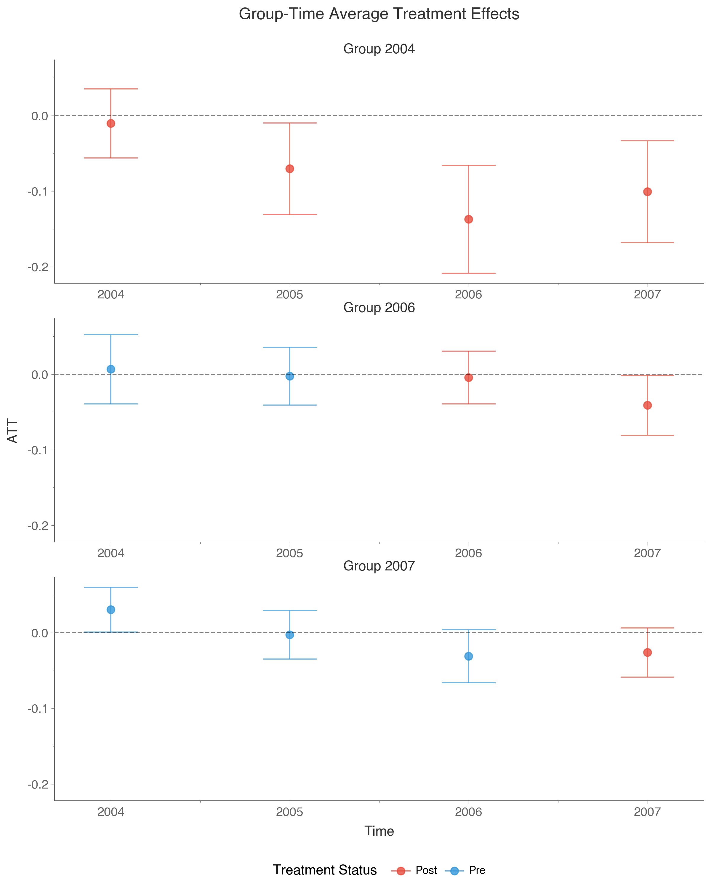

While group-time effects are useful, they can be difficult to summarize when there are many groups and time periods. The aggte function aggregates these into more interpretable summaries. Setting type="dynamic" produces an event study that shows how effects evolve relative to treatment timing:

event_study = did.aggte(result, type="dynamic")
print(event_study)

==============================================================================
Aggregate Treatment Effects (Event Study)
==============================================================================

Overall summary of ATT's based on event study/dynamic aggregation:

┌─────────┬────────────┬────────────────────────┐
│     ATT │ Std. Error │ [95% Conf. Interval]   │
├─────────┼────────────┼────────────────────────┤
│ -0.0042 │     0.0119 │ [ -0.0275,   0.0191]   │
└─────────┴────────────┴────────────────────────┘


Dynamic Effects:

┌────────────┬──────────┬────────────┬──────────────────────────┐
│ Event time │ Estimate │ Std. Error │ [95% Simult. Conf. Band] │
├────────────┼──────────┼────────────┼──────────────────────────┤
│         -3 │  -0.0031 │     0.0161 │ [-0.0445,  0.0383]       │
│         -2 │  -0.0046 │     0.0175 │ [-0.0499,  0.0406]       │
│         -1 │   0.0000 │         NA │ NA                       │
│          0 │  -0.0212 │     0.0162 │ [-0.0629,  0.0204]       │
│          1 │   0.0264 │     0.0333 │ [-0.0596,  0.1124]       │
│          2 │  -0.0232 │     0.0204 │ [-0.0758,  0.0293]       │
│          3 │   0.0311 │     0.0255 │ [-0.0346,  0.0967]       │
└────────────┴──────────┴────────────┴──────────────────────────┘

------------------------------------------------------------------------------
Signif. codes: '*' confidence band does not cover 0

------------------------------------------------------------------------------
Data Info
------------------------------------------------------------------------------
Control group: Not yet treated

------------------------------------------------------------------------------
Estimation Details
------------------------------------------------------------------------------
Estimation method: Doubly Robust (dr)
Base period: Varying
Anticipation periods: 0

------------------------------------------------------------------------------
Inference
------------------------------------------------------------------------------
Significance level: 0.05
Bootstrap iterations: 999
Bootstrap type: Weighted
==============================================================================
Reference: Callaway and Sant'Anna (2021)

Event time 0 is the period of first treatment, e.g., the on-impact effect, negative event times are pre-treatment periods, and positive event times are post-treatment periods. Pre-treatment effects near zero lean in support of the parallel trends assumption (but do not confirm it), while post-treatment effects reveal how the treatment impact evolves over time. The overall ATT at the top provides a single summary measure across all post-treatment periods.

We can also use built-in plotting functionality to plot the event study results with plot_event_study():

did.plot_event_study(event_study)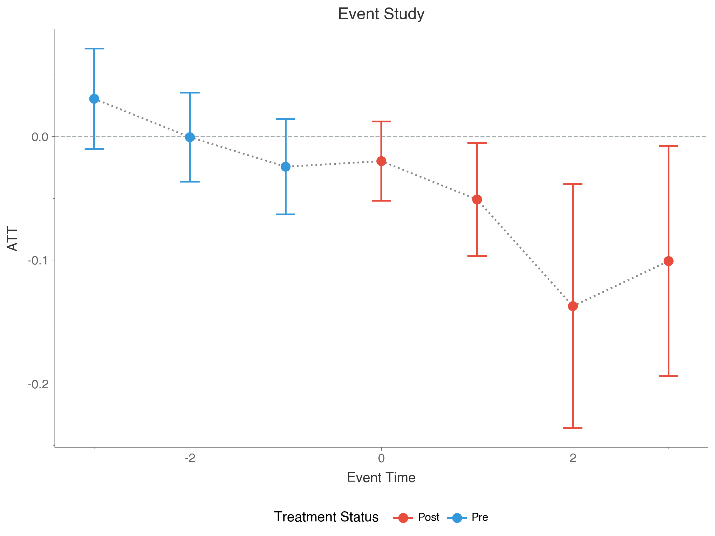

Common Troubleshooting for GPU

If set_backend("cupy") raises CuPy is not installed, the most common cause is installing the generic cupy package, which tries to compile from source. Instead, install a prebuilt wheel that matches your CUDA driver version:

uv pip install cupy-cuda12x   # CUDA 12.x
uv pip install cupy-cuda11x   # CUDA 11.x

Run nvidia-smi to check which CUDA version your driver supports. After installing, restart your Python process (or notebook runtime) before importing ModernDiD (CuPy availability is checked once at import time).

If you see cudaErrorInsufficientDriver, the installed CuPy wheel expects a newer CUDA version than your driver provides. Check nvidia-smi and switch to the matching wheel.

If you see No CUDA GPU is available, make sure nvidia-smi shows a device. In cloud notebooks, verify that a GPU runtime is selected.

Available Methods

Each core module includes a dedicated walkthrough covering methodology background, API usage, and guidance on interpreting results.

Core Implementations

Module	Description	Reference
moderndid.did	Staggered DiD with group-time effects	Callaway & Sant'Anna (2021)
moderndid.drdid	Doubly robust 2-period estimators	Sant'Anna & Zhao (2020)
moderndid.didhonest	Sensitivity analysis for parallel trends	Rambachan & Roth (2023)
moderndid.didcont	Continuous/multi-valued treatments	Callaway et al. (2024)
moderndid.didtriple	Triple difference-in-differences	Ortiz-Villavicencio & Sant'Anna (2025)
moderndid.didinter	Intertemporal DiD with non-absorbing treatment	Chaisemartin & D'Haultfœuille (2024)

Planned Development

Module	Description	Reference
moderndid.didml	Machine learning approaches to DiD	Hatamyar et al. (2023)
moderndid.drdidweak	Robust to weak overlap	Ma et al. (2023)
moderndid.didcomp	Compositional changes in repeated cross-sections	Sant'Anna & Xu (2025)
moderndid.didimpute	Imputation-based estimators	Borusyak, Jaravel, & Spiess (2024)
moderndid.didbacon	Goodman-Bacon decomposition	Goodman-Bacon (2019)
moderndid.didlocal	Local projections DiD	Dube et al. (2025)
moderndid.did2s	Two-stage DiD	Gardner (2021)
moderndid.etwfe	Extended two-way fixed effects	Wooldridge (2021), Wooldridge (2023)
moderndid.functional	Specification tests	Roth & Sant'Anna (2023)